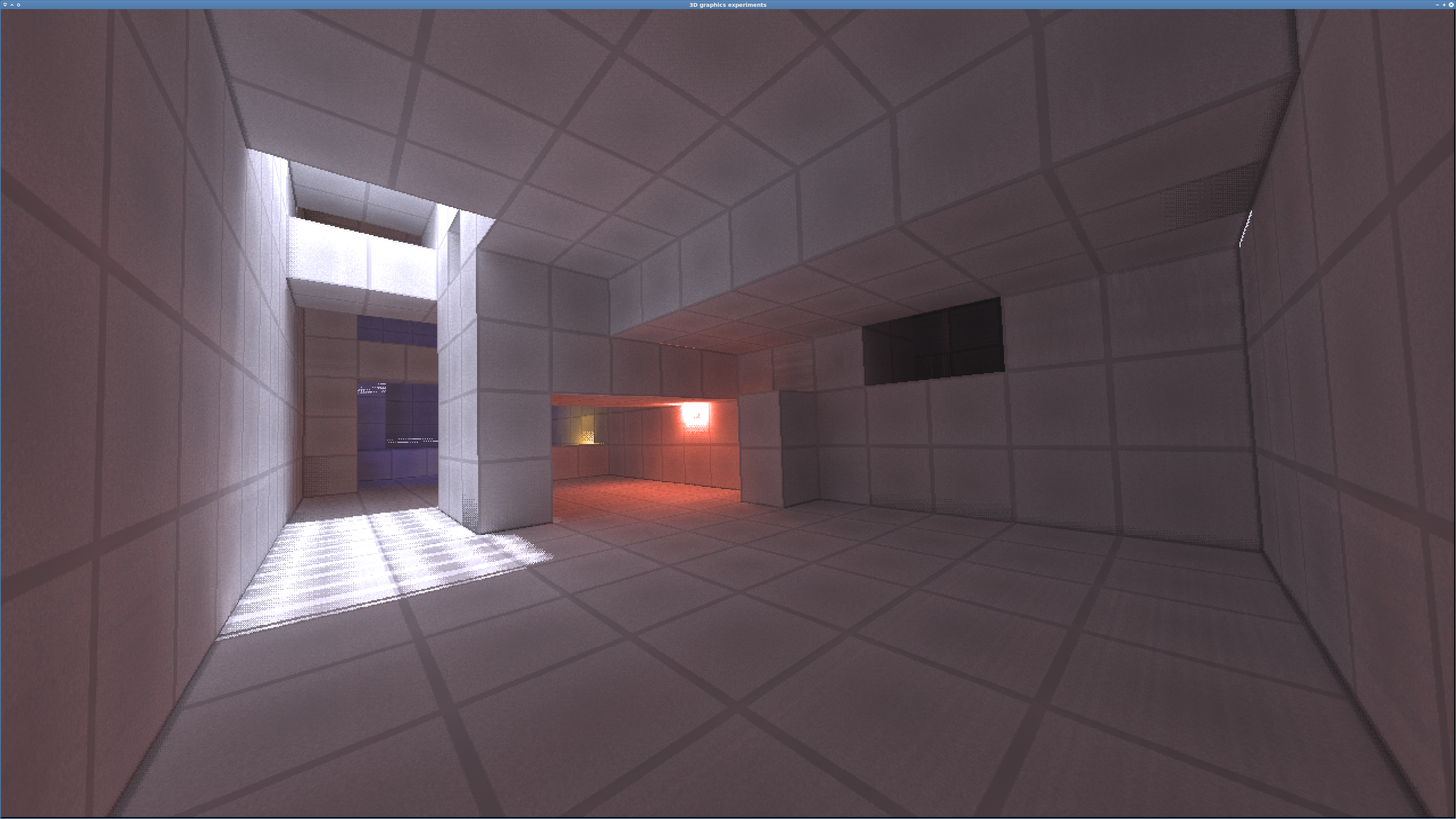
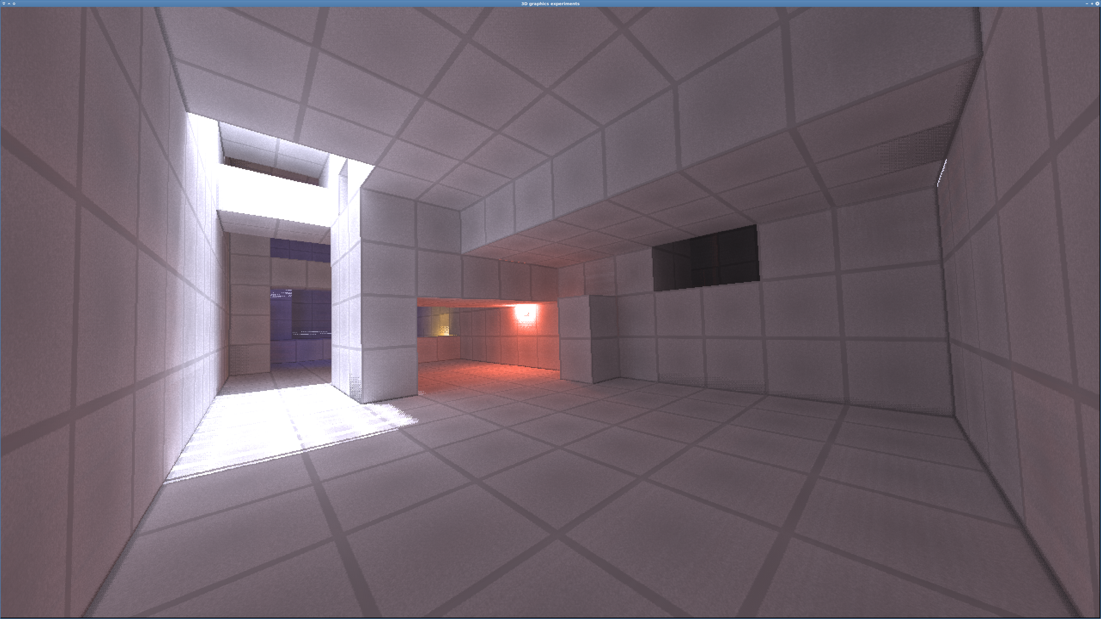
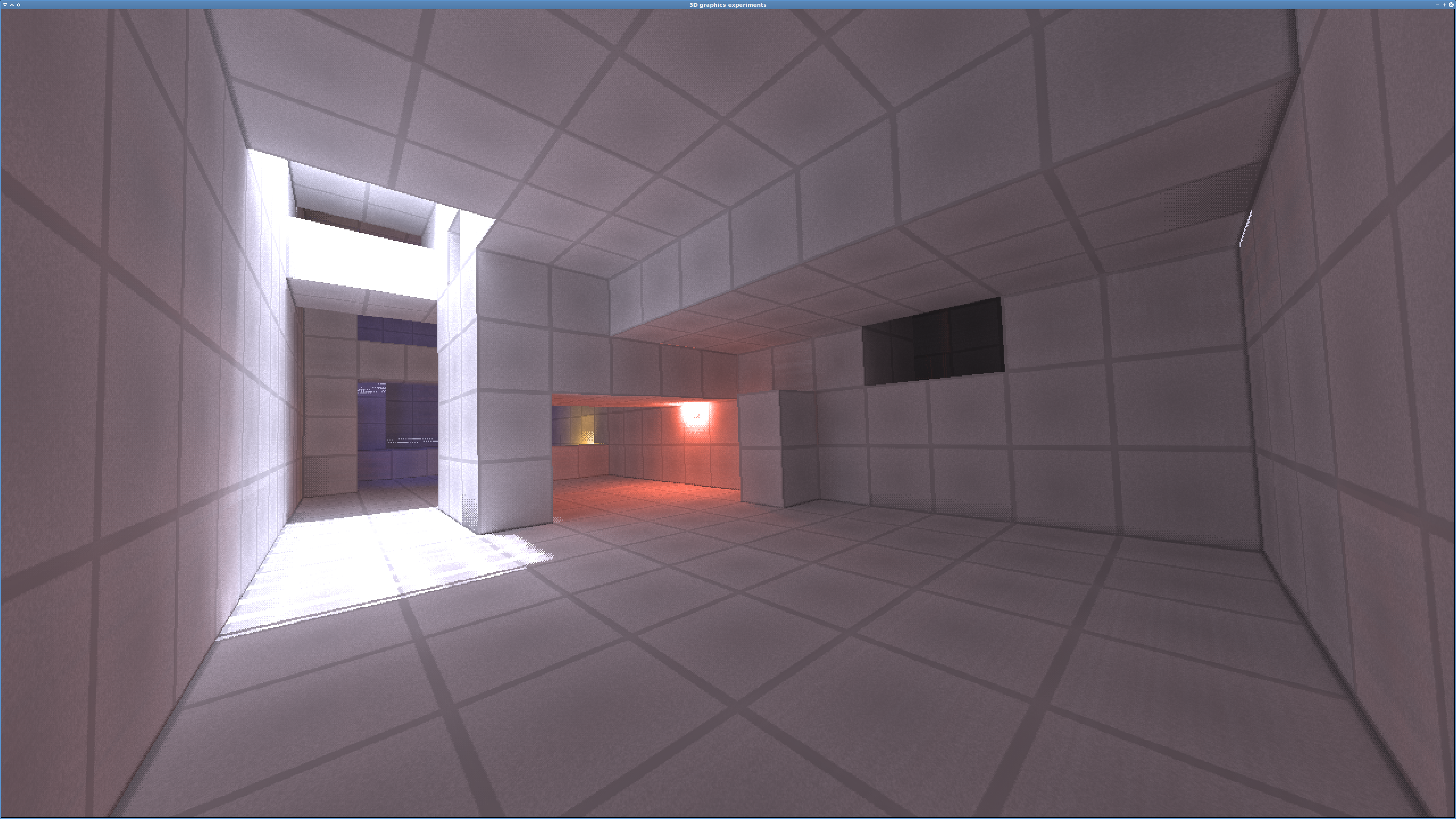
No workaround — Beams visible

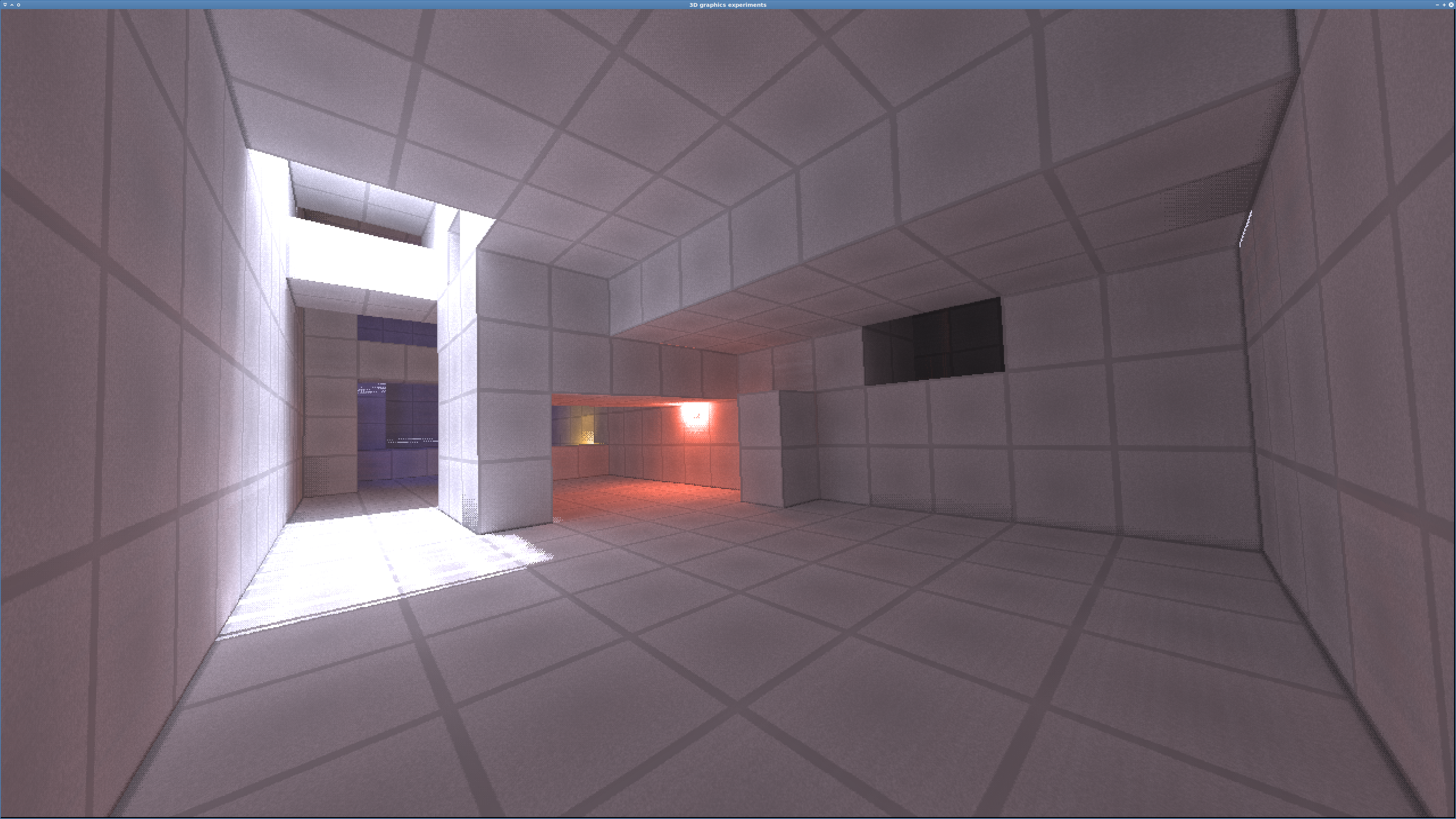
Workaround 1 — Looks fine to me

angle  = acos(view_vector.z)
diff   = abs(tan(angle) − tan(angle + 0.01)) // Width of an angular band of 0.01 radians
adjust = 1 / diff

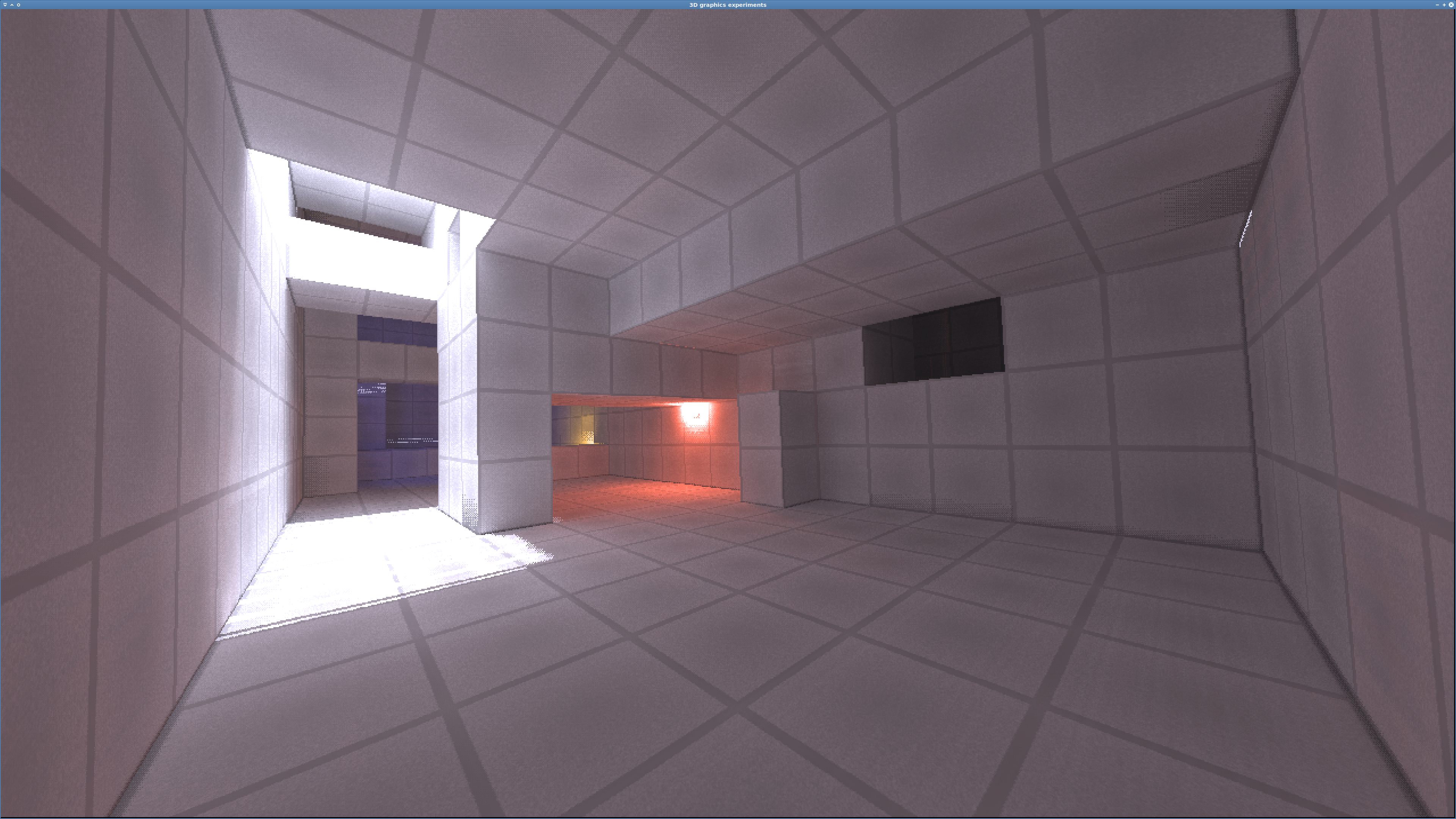
Workaround 2 — Looks indistinguishable from workaround 1

diff   = abs(tan(angle) − tan(angle + 0.1)) // Width of an angular band of 0.1 radians
adjust = 1 / diff

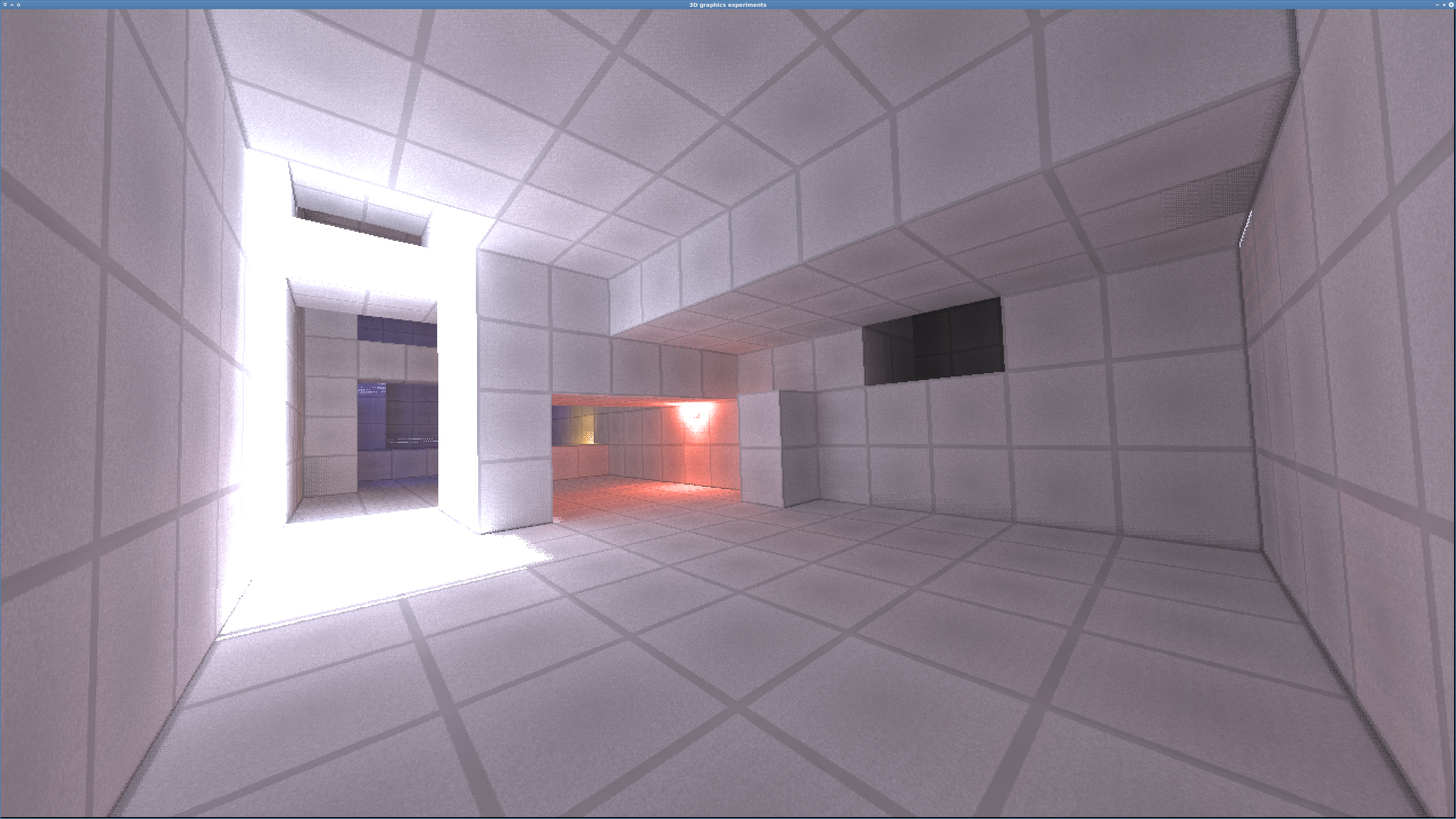
Workaround 3 (bad)

vx       = view_vector.x / view_vector.z
vy       = view_vector.y / view_vector.z
radius   = sqrt(vx*vx + vy*vy)        // distance of the projected pixel from the view center
constant = 2 * π
area     = constant * radius*radius   // number of pixels inside this radius
area     = constant * (vx*vx + vy*vy) // faster way to calculate the same
adjust   = 1 / (1 + area)

Here the compensation is too powerful, and there are now horizontal and vertical beams instead of diagonal ones

Workaround 4 — Looks indistinguishable from workarounds 1 and 2

area     = vx*vx + vy*vy              // Ignore the constant
adjust   = 1 / (1 + area)             // Still don’t understand how to justify the 1 in “1 + ”, but it seems to work — why not 5? Why not 0.001?

Workaround 5 — Just testing

diff   = abs(tan(angle) − tan(angle + 10⁻⁶)) // Width of an angular band of 0.000001 radians
adjust = 1 / diff

Looks like the choice of the constant used in the tan calculation is not particularly important.

Conclusion

The weight for each sample can be calculated as follows:

Vz     = view_vector.z
angle  = acos(Vz)
band   = 0.0001                            // Radians. Any number between 10⁻⁵ and 10⁻³ seems to work fine
diff   = abs(tan(angle) − tan(angle+band)) // Width of an angular band
adjust = 1 / diff
power  = max(0, normal · view_vector)      // This is the cosine (Lambertian reflectance)
weight = power * adjust   // This is the adjusted cosine, accounting for edge skew caused by rectilinear projection

However, the following calculation produces identical results with much cheaper operations:

Vx     = view_vector.x
Vy     = view_vector.y
vx     = Vx / Vz
vy     = Vy / Vz
area   = vx*vx + vy*vy
adjust = 1 / (1 + area)
weight = power * adjust   // This is the adjusted cosine, accounting for edge skew caused by rectilinear projection

After asking Maxima to simplify (Vx/Vz)^2 + (Vy/Vz)^2, I discovered that the above calculation can be simplified to:

area = (Vx*Vx + Vy*Vy) / (Vz*Vz)           // Saves one division

and then, after asking it about 1 / (1 + (Vx*Vx+Vy*Vy)/(Vz*Vz)), I discovered this alternative:

adjust = Vz*Vz / (Vx*Vx + Vy*Vy + Vz*Vz)   // Saves two divisions

and because I knew that view_vector just happens to be a unit vector,

adjust = Vz*Vz                             // Saves all divisions

so the final result is:

power  = max(0, normal · view_vector)      // This is the cosine (Lambertian reflectance)
Vz     = view_vector.z
weight = power * Vz*Vz    // This is the adjusted cosine, accounting for edge skew caused by rectilinear projection

That is way simpler than I expected.

Why though?

Let’s simplify

adjust = 1 / abs(tan(acos(Vz)) − tan(acos(Vz)+band))

Why does this lead into the same result as this?

adjust = someconstant * Vz * Vz

According to definition…

acos(x) = atan(sqrt(1−x²) / x)

So,

tan(acos(x)) = sqrt(1−x²) / x

So the goal we want to figure out is:

abs(sqrt(1−x²) / x − sqrt(1−(x+band)²) / (x+band)) = someconstant * x²

What is the relationship between band and someconstant?